クエリプランナーの内側:Amazon NeptuneのEXPLAINプランを読み解く

リレーショナルデータベースとは異なり、グラフクエリは多数のエッジをまたぐトラバーサル、動的なフィルタリング、パターンマッチングを伴うことが多くあります。そのためパフォーマンスの予測が難しく、従来のインデックス戦略がそのまま通用しないこともあります。そこで活躍するのがクエリプランナーです。Neptuneがクエリをどう解釈し、どこで時間を浪費している可能性があるのかを教えてくれます。

サポートされている各言語でEXPLAINプランを生成する方法を見ていきましょう。

GremlinでPROFILEプランを生成するには、Neptune WorkbenchやNeptune拡張に対応したGremlin互換プロンプトから、profile HTTPエンドポイントを呼び出します。EXPLAINではなくPROFILEを使うとクエリが実際に実行されるため、より価値のある統計情報が得られます。

POST https://<your-neptune-endpoint>:<port>/gremlin/profile \
     -d '{
           "gremlin":"g.V().hasLabel(\"city\")
                               .has(\"name\", \"London\")
                               .emit()
                               .repeat(in().simplePath())
                               .times(2)
                               .limit(100)"
        }'

Jupyter Notebookで実行する場合は、以下のマジックセルコマンドも利用できます。

%%gremlin profile

これによりクエリが実行され、以下を含む完全なプロファイルレポートが返されます。

• 実行ステップ
• 所要時間とカウント
• 最適化済みプランおよび物理クエリプラン
• トラバーサルおよびリピートのメトリクス

出力サンプル(分かりやすさのため一部省略):

Query String
==================
g.V().hasLabel("city").has("name", "London").emit().repeat(in().simplePath()).times(2).limit(100)Original Traversal
==================
[GraphStep(vertex,[]), HasStep([...]), RepeatStep(...), RangeGlobalStep(0,100)]Optimized Traversal
===================
Neptune steps:
[\
  NeptuneGraphQueryStep(Vertex) {\
    JoinGroupNode {\
      PatternNode[(?1, <name>, "London", ?) . project ?1 .], {...}\
      PatternNode[(?1, <~label>, ?2=<city>, <~>) . project ask .], {...}\
      RepeatNode {\
        Repeat {\
          PatternNode[(?3, ?5, ?1, ?6) . project ?1,?3 . SimplePathFilter(?1, ?3)) .], {...}\
        }\
        Emit { Filter(true) }\
        LoopsCondition { LoopsFilter([?1, ?3], eq(2)) }\
      }\
    }, finishers=[limit(100)]\
  },\
  NeptuneTraverserConverterStep\
]Physical Pipeline
=================
NeptuneGraphQueryStep
  |-- JoinGroupOp
      |-- DynamicJoinOp(...)
      |-- RepeatOp
          |-- BindingSetQueue (Iteration 1)...
          |-- BindingSetQueue (Iteration 2)...
  |-- LimitOp(100)Runtime (ms)
============
Query Execution:  392.686
Serialization:   2636.380Traversal Metrics
=================
Step                            Count  Traversers   Time (ms)    % Dur
--------------------------------------------------------------
NeptuneGraphQueryStep(Vertex)    100         100      314.162    82.78
NeptuneTraverserConverterStep    100         100       65.333    17.22
TOTAL                               -           -      379.495       -Repeat Metrics
==============
Iteration  Visited   Output    Until     Emit     Next
------------------------------------------------------
        0        1        1        0        1        1
        1       61       61        0       61       61
        2       38       38       38        0        0
------------------------------------------------------
              100      100       38       62       62Results
=======
Count: 100
Response size (bytes): 23566

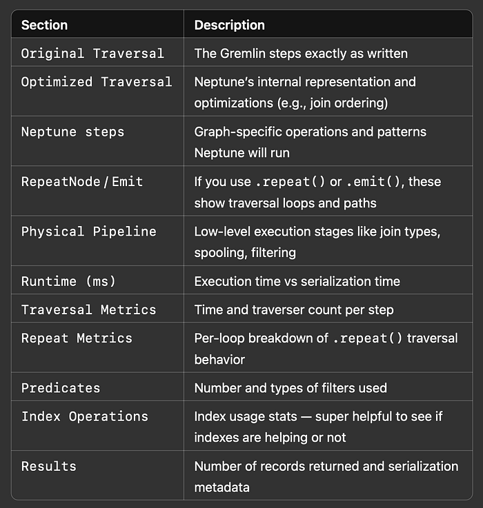
各セクションが何を示しているのか、要点を整理しておきましょう。

SPARQLではクエリと一緒に explain=details パラメータを指定します。curl を使って詳細なEXPLAINプランを取得する例は次のとおりです(Jupyterで実行する場合はマジックセルコマンドも利用できます)。

curl https://<your-neptune-endpoint>:<port>/sparql \
  -d "query=PREFIX ex: <https://example.com/> \
      SELECT ?person WHERE { ?person a ex:City ; ex:name \"London\" }" \
  -d "explain=details"

出力サンプル:

╔════╤════════╤════════╤═══════════════════╤═══════════════════════════════════════════════════════╤══════════╤══════════╤═══════════╤═══════╤═══════════╗
║ ID │ Out #1 │ Out #2 │ Name              │ Arguments                                             │ Mode     │ Units In │ Units Out │ Ratio │ Time (ms) ║
╠════╪════════╪════════╪═══════════════════╪═══════════════════════════════════════════════════════╪══════════╪══════════╪═══════════╪═══════╪═══════════╣
║ 0  │ 1      │ -      │ SolutionInjection │ solutions=[{}]                                        │ -        │ 0        │ 1         │ 0.00  │ 0         ║
╟────┼────────┼────────┼───────────────────┼───────────────────────────────────────────────────────┼──────────┼──────────┼───────────┼───────┼───────────╢
║ 1  │ 2      │ -      │ PipelineJoin      │ pattern=distinct(?person, rdf:type, ex:City)          │ -        │ 1        │ 2         │ 2.00  │ 1         ║
╟────┼────────┼────────┼───────────────────┼───────────────────────────────────────────────────────┼──────────┼──────────┼───────────┼───────┼───────────╢
║ 2  │ 3      │ -      │ PipelineJoin      │ pattern=distinct(?person, ex:name, \"London\")        │ -        │ 2        │ 2         │ 1.00  │ 1         ║
╟────┼────────┼────────┼───────────────────┼───────────────────────────────────────────────────────┼──────────┼──────────┼───────────┼───────┼───────────╢
║ 3  │ 4      │ -      │ Projection        │ vars=[?person]                                        │ retain   │ 2        │ 2         │ 1.00  │ 0         ║
╟────┼────────┼────────┼───────────────────┼───────────────────────────────────────────────────────┼──────────┼──────────┼───────────┼───────┼───────────╢
║ 4  │ -      │ -      │ TermResolution    │ vars=[?person]                                        │ id2value │ 2        │ 2         │ 1.00  │ 1         ║
╚════╧════════╧════════╧═══════════════════╧═══════════════════════════════════════════════════════╧══════════╧══════════╧═══════════╧═══════╧═══════════╝

explain=details は、SPARQLクエリがNeptune内部でどのように計画・実行されるのかを最も詳しく把握できる手段です。

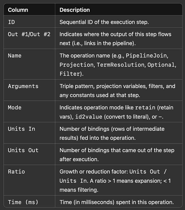
各セクションが何を示しているのか、要点を整理しておきましょう。

openCypherでEXPLAINプランを生成するには、explain=details パラメータを使用します(Jupyterで実行する場合はマジックセルコマンドも利用できます)。

curl https://<your-neptune-endpoint>:<port>/openCypher \
  -d "query=MATCH (c:City {name: 'London'}) RETURN c" \
  -d "explain=details"

出力サンプル:

Query:
MATCH (c:City {name: 'London'}) RETURN c
╔════╤════════╤════════╤═══════════════════╤════════════════════╤═════════════════════╤══════════╤═══════════╤═══════╤═══════════╗
║ ID │ Out #1 │ Out #2 │ Name              │ Arguments          │ Mode                │ Units In │ Units Out │ Ratio │ Time (ms) ║
╠════╪════════╪════════╪═══════════════════╪════════════════════╪═════════════════════╪══════════╪═══════════╪═══════╪═══════════╣
║ 0  │ 1      │ -      │ SolutionInjection │ solutions=[{}]     │ -                   │ 0        │ 1         │ 0.00  │ 0         ║
╟────┼────────┼────────┼───────────────────┼────────────────────┼─────────────────────┼──────────┼───────────┼───────┼───────────╢
║ 1  │ 2      │ -      │ DFESubquery       │ subQuery=subQuery1 │ -                   │ 0        │ 10        │ 0.00  │ 5.00      ║
╟────┼────────┼────────┼───────────────────┼────────────────────┼─────────────────────┼──────────┼───────────┼───────┼───────────╢
║ 2  │ -      │ -      │ TermResolution    │ vars=[?c]          │ id2value_opencypher │ 10       │ 10        │ 1.00  │ 1.00      ║
╚════╧════════╧════════╧═══════════════════╧════════════════════╧═════════════════════╧══════════╧═══════════╧═══════╧═══════════╝subQuery1:
╔════╤════════╤════════╤═════════════════╤═══════════════════════════════════════════════════════════╤══════╤══════════╤═══════════╤═══════╤═══════════╗
║ ID │ Out #1 │ Out #2 │ Name            │ Arguments                                                 │ Mode │ Units In │ Units Out │ Ratio │ Time (ms) ║
╠════╪════════╪════════╪═════════════════╪═══════════════════════════════════════════════════════════╪══════╪══════════╪═══════════╪═══════╪═══════════╣
║ 0  │ 1      │ -      │ DFEPipelineScan │ pattern=Node((?anon_node)-[:?rel]->())                   │ -    │ 0        │ 1000      │ 0.00  │ 0.66      ║
║    │        │        │                 │ inlineFilters=[(?label = :City), (?name = 'London')]     │      │          │           │       │           ║
╟────┼────────┼────────┼─────────────────┼───────────────────────────────────────────────────────────┼──────┼──────────┼───────────┼───────┼───────────╢
║ 1  │ 2      │ -      │ DFEProject      │ columns=[?c]                                              │ -    │ 1000     │ 1000      │ 1.00  │ 0.14      ║
╟────┼────────┼────────┼─────────────────┼───────────────────────────────────────────────────────────┼──────┼──────────┼───────────┼───────┼───────────╢
║ 2  │ -      │ -      │ DFEDrain        │ limit=10                                                  │ -    │ 1000     │ 0         │ 0.00  │ 0.11      ║
╚════╧════════╧════════╧═════════════════╧═══════════════════════════════════════════════════════════╧══════╧══════════╧═══════════╧═══════╧═══════════╝

openCypherの explain=details は、実行ステージ、ジョインの構造、上限値、パターンの推定値などを表形式で示します。標準出力よりもパフォーマンス分析に格段に役立ちます。

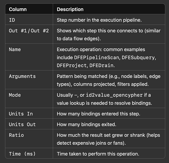
各セクションが何を示しているのか、要点を整理しておきましょう。

GremlinのPROFILE出力は、実行ステージとそのコストの内訳を示します。なかでもRepeat Metricsはトラバーサルループの理解に有用で、ループはグラフクエリで頻発するパフォーマンスの落とし穴です。コストの高いトラバーサル区間を特定し、フィルタやパスのロジックが実行にどう影響しているかを把握できます。

SPARQLとopenCypherでは、details モードを使うことで静的なプランがステップ単位の詳細な分析へと変わります。ジョインの種類、プロジェクションの順序、フィルタ、オペレータごとの処理時間、推定値と実測値のデータ量比較といった情報が得られます。

シンプルなGremlinクエリを例に解説します。このクエリはロンドン市を表すノードから出発し、入ってくるすべての接続を最大3ステップ遡ってたどります(同じノードを2度通らないように制御)。次にたどり着いた各ノードから1ステップ先へ進んで接続先のノードを取得し、その中から「event」タイプのもののみ(=type プロパティが「event」のノード)を抽出。最後に最大50件の結果を返します。Gremlinで書くと次のようになります。

g.V()
  .has("name", "London")
  .hasLabel("city")
  .repeat(in().simplePath())
  .times(3)
  .out()
  .has("type", "event")
  .limit(50)

Explainプラン:

*******************************************************
                Neptune Gremlin Profile
*******************************************************

Query String
==================
g.V().has("name", "London").hasLabel("city").repeat(in().simplePath()).times(3).out().has("type", "event").limit(50)

Original Traversal
==================

Optimized Traversal
===================
Neptune steps:
[\
  NeptuneGraphQueryStep(Vertex) {\
    JoinGroupNode {\
      PatternNode[(?1, <name>, "London", ?) . project ?1 .], {estimatedCardinality=2, indexTime=75, joinTime=4, hashJoin=true, actualTotalOutput=2} [1]\
      PatternNode[(?1, <~label>, ?2=<city>, <~>) . project ask .], {estimatedCardinality=10000, indexTime=33, hashJoin=true, joinTime=0, actualTotalOutput=2} [1]\
      RepeatNode {\
        Repeat {\
          PatternNode[(?3, ?5, ?1, ?6) . project ?1,?3 . IsEdgeIdFilter(?6) . SimplePathFilter(?1, ?3)) .], {estimatedCardinality=70000, hashJoin=true, indexTime=0, joinTime=5} [2]\
        }\
        Emit {\
          Filter(false)\
        }\
        LoopsCondition {\
          LoopsFilter([?1, ?3],eq(3))\
        }\
      }, annotations={repeatMode=BFS, emitFirst=false, untilFirst=false, leftVar=?1, rightVar=?3}\
    }, finishers=[filter(type=event), limit(50)], annotations={path=[Vertex(?1):GraphStep, Repeat[Vertex(?3):VertexStep], Vertex(?4):VertexStep], joinStats=true, optimizationTime=519, maxVarId=9, executionTime=483} [3]\
  },\
  NeptuneTraverserConverterStep\
]

Physical Pipeline
=================
NeptuneGraphQueryStep
  |-- StartOp
  |-- JoinGroupOp
      |-- SpoolerOp(100)
      |-- DynamicJoinOp(PatternNode[(?1, <name>, "London", ?) . project ?1 .], {estimatedCardinality=2, indexTime=75}) [1]
      |-- SpoolerOp(100)
      |-- DynamicJoinOp(PatternNode[(?1, <~label>, ?2=<city>, <~>) . project ask .], {estimatedCardinality=10000, indexTime=33}) [1]
      |-- RepeatOp
          |-- <upstream input> (Iteration 0) [visited=2, output=2 (until=0, emit=0), next=2]
          |-- BindingSetQueue (Iteration 1) [visited=250, output=250 (until=0, emit=0), next=250]
              |-- DynamicJoinOp(PatternNode[(?3, ?5, ?1, ?6) . ...]) [2]
          |-- BindingSetQueue (Iteration 2) [visited=950, output=950 (until=0, emit=0), next=950]
          |-- BindingSetQueue (Iteration 3) [visited=19500, output=19500 (until=19500, emit=0), next=0]
      |-- VertexStep(OUT)
      |-- FilterStep(type = event) [3]
      |-- LimitOp(50)

Runtime (ms)
============
Query Execution: 483.222
Serialization:   2798.304

Traversal Metrics
=================
Step                            Count  Traversers   Time (ms)
------------------------------------------------------------
NeptuneGraphQueryStep           50        50        403.187
NeptuneTraverserConverterStep  50        50         80.035

Repeat Metrics
==============
Iteration  Visited   Output    Until     Emit     Next
------------------------------------------------------
        0        2        2        0        0        2
        1      250      250        0        0      250
        2      950      950        0        0      950
        3    19500    19500    19500        0        0
------------------------------------------------------
            20702    20702    19500        0     1202

Warnings:
⚠ reverse traversal with no edge label(s) [2]
⚠ high fan-out detected in repeat [2]
⚠ filter applied late in traversal chain [3]

EXPLAINプランから読み取れること

[x] は、上記のexplainプラン内で対応する箇所を示しています。

• [1] 非効率な開始:カーディナリティは低いものの、絞り込み効率を高めるために2つのフィルタを並べ替える余地があります。カーディナリティが高いほどデータ内で取り得る値の幅が広く、結果として一致する値が少なくなるため、返されるデータ量は小さくなります。狙うべきは、最も小さなデータセットを最初に得ることです。たとえば、最大10,000ノードに作用するフィルタが2つあるとします。一方は50%、もう一方は10%のノードを選択するとしましょう。10%のフィルタを先に処理すれば、次のフィルタへ渡るのは1,000ノードだけで済みます。逆順だと次のフィルタには5倍のノードが渡され、処理量が増えてクエリが遅くなります。
• [2] .in() にエッジラベルが指定されていないため、すべての受信エッジをスキャンすることになります。リピートトラバーサルのサイズが2件から約2万ノードへと爆発的に膨れ上がっています。
• [3] .out() と .has("type", "event") のフィルタが、この大規模な展開の後に適用されており非効率です。
• 合計トラバーサル件数:2万件以上。多くの処理が無駄になっています。

g.V()
  .hasLabel("city")
  .has("name", "London")
  .repeat(in("located_in").simplePath())
  .times(3)
  .out("hosts")
  .has("type", "event")
  .limit(50)

• .in() と .out() の両方にエッジラベルフィルタを追加
• .has("type", "event") を前倒しし、後続処理のコストを削減
• .simplePath() はサイクル防止のため残しつつ、テスト時には任意で外せるよう対応

*******************************************************
                Neptune Gremlin Profile
*******************************************************

Query String
==================
g.V().hasLabel("city").has("name", "London")
  .repeat(in("located_in").simplePath()).times(3)
  .out("hosts").has("type", "event").limit(50)

Original Traversal
==================
[GraphStep(vertex,[]),\
 HasStep([~label.eq(city)]),\
 HasStep([name.eq(London)]),\
 RepeatStep(emit(false), [VertexStep(IN,[located_in]), PathFilterStep(simple), RepeatEndStep], until(loops(3))),\
 VertexStep(OUT,[hosts]),\
 HasStep([type.eq(event)]),\
 RangeGlobalStep(0,50)]

Optimized Traversal
===================
Neptune steps:
[\
  NeptuneGraphQueryStep(Vertex) {\
    JoinGroupNode {\
      PatternNode[(?1, <~label>, ?2=<city>, <~>) . project ask .], {estimatedCardinality=3000, indexTime=21, actualTotalOutput=7}\
      PatternNode[(?1, <name>, "London", ?) . project ?1 .], {estimatedCardinality=1, indexTime=62, actualTotalOutput=1}\
      RepeatNode {\
        Repeat {\
          PatternNode[(?3, <located_in>, ?1, ?) . project ?1,?3 . SimplePathFilter(?1,?3)] {estimatedCardinality=4500, hashJoin=true}\
        }\
        Emit { Filter(false) }\
        LoopsCondition { LoopsFilter([?1, ?3], eq(3)) }\
      }, annotations={repeatMode=BFS, emitFirst=false, untilFirst=false, leftVar=?1, rightVar=?3}\
    },\
    JoinGroupNode {\
      PatternNode[(?3, <hosts>, ?4, ?) . project ?4 .], {estimatedCardinality=500, hashJoin=true}\
      PatternNode[(?4, <type>, "event", ?) . project ?4 .], {estimatedCardinality=150, hashJoin=true}\
    },\
    finishers=[limit(50)],\
    annotations={executionTime=192, optimizationTime=87, path=[Vertex(?1)->Repeat(?3)->Vertex(?4)]}\
  },\
  NeptuneTraverserConverterStep\
]

Physical Pipeline
=================
NeptuneGraphQueryStep
  |-- StartOp
  |-- JoinGroupOp
      |-- DynamicJoinOp(PatternNode[(?1, <~label>, ?2=<city>, <~>) ...])
      |-- DynamicJoinOp(PatternNode[(?1, <name>, "London", ?) ...])
      |-- RepeatOp
          |-- Iteration 0: visited=1, output=1, next=1
          |-- Iteration 1: visited=35, output=35, next=35
          |-- Iteration 2: visited=85, output=85, next=85
          |-- Iteration 3: visited=120, output=120, next=0
      |-- DynamicJoinOp(PatternNode[(?3, <hosts>, ?4, ?) ...])
      |-- DynamicJoinOp(PatternNode[(?4, <type>, "event", ?) ...])
      |-- LimitOp(50)

Runtime (ms)
============
Query Execution: 172.329
Serialization:    817.502

Traversal Metrics
=================
Step                            Count  Traversers   Time (ms)   % Dur
---------------------------------------------------------------------
NeptuneGraphQueryStep            50        50         139.438   80.9
NeptuneTraverserConverterStep    50        50          32.891   19.1
                                TOTAL                  172.329

Repeat Metrics
==============
Iteration  Visited   Output    Until     Emit     Next
------------------------------------------------------
        0        1        1        0        0        1
        1       35       35        0        0       35
        2       85       85        0        0       85
        3      120      120        0        0        0
------------------------------------------------------
              241      241        0        0      121

Predicates
==========
# of predicates: 10

Results
=======
Count: 50
Output: [v[302], v[417], v[501], v[519], v[520], v[622], v[635], v[780], v[801], ...]
Response serializer: GRYO_V3D0
Response size (bytes): 18310

Index Operations
================
Query execution:
    # of statement index ops: 4
    # of unique statement index ops: 4
    Duplication ratio: 1.00
    # of terms materialized: 0

Serialization:
    # of statement index ops: 100
    # of unique statement index ops: 88
    Duplication ratio: 1.14
    # of terms materialized: 145

• 総トラバーサルノード数:約886件 vs 約20,702件
• クエリ時間が60%以上短縮
• メモリ負荷とタイムアウトリスクの低減

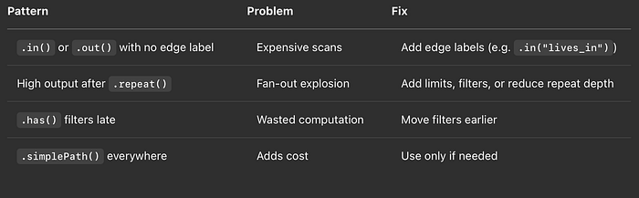
EXPLAINプランで押さえるべき主要領域をまとめた表

• フィルタはプッシュダウン:できるだけクエリの早い段階でフィルタを適用しましょう。
• 方向の選択を工夫する:出発点をより絞り込めるなら、トラバーサルの方向を逆にすることも検討してください。
• OPTIONAL(SPARQL)には注意:プランの複雑さを大幅に増やす可能性があります。
• ラベルのカーディナリティを意識する:高カーディナリティのラベルはクエリの起点として好パフォーマンスを発揮します。
• モデル設計も忘れずに:パフォーマンス問題は、グラフ構造そのものの設計が原因のこともあります。

大規模なプランを扱う場合は、JSON出力をパースしてGraphvizやD3.jsでツリー表示するPythonスクリプトを書くのもおすすめです。構造を理解しやすくなり、チームメンバーとの共有にも役立ちます。