Cloud Intelligence™
Why Your Amazon Redshift Concurrency Scaling Costs Keep Growing (And How to Fix It)
This page is also available in Deutsch, Español, Français, Italiano, 日本語, and Português.


About Joseph Allam
Databases have been my craft for a long time — long before the cloud, and deep into it across AWS and GCP. I know what breaks, what costs too much, and what needs rethinking before it hurts. I also know how to bring AI into the work: into how databases are designed, operated, and accessed by the intelligent systems being built on top of them.
My personal pageUnexpected Amazon Redshift cost increases often look like isolated spikes at first. In practice, they are usually caused by workload patterns that quietly push Concurrency Scaling beyond its intended role.
Concurrency Scaling is designed to add Redshift capacity when query demand increases, and to remove that capacity when demand subsides. It is useful for bursts. When it becomes active for long periods, though, it starts behaving less like overflow capacity and more like baseline compute. That usually changes the cost profile of the workload.
This post walks through a real-world style Redshift investigation where elevated spend initially looked like normal workload growth. A closer review of billing data, cluster configuration, and CloudWatch metrics showed a different pattern: mixed workloads were sharing the same cluster, creating sustained CPU pressure, and triggering Concurrency Scaling for most of the day.
We'll walk through the investigation, the metrics that mattered, the configuration choices that amplified cost, and the remediation plan.
PerfectScale™ for Kubernetes
Ready to optimize?
Get your free Kubernetes savings analysis
What you'll get from this write-up
By the end, you should have a practical workflow for:
- Identifying which Redshift cluster is driving cost
- Separating CPU pressure from queueing pressure
- Spotting when Concurrency Scaling is being used as baseline capacity
- Catching WLM routing issues that amplify cost
- Building a phased remediation plan
Step 1: Confirm the cost driver before changing anything
When Redshift costs rise unexpectedly, the temptation is to jump straight into query tuning or cluster resizing. That is risky. Query tuning can help, and resizing may eventually be needed, but neither should be the first move.
The first question is simpler:
Which Redshift resource is actually responsible for the increase?
In this investigation the environment had two provisioned Redshift clusters:
| Cluster | Role | Cost behaviour |
|---|---|---|
analytics-production-cluster |
Main analytics, BI, application, batch, and ML workloads | High cost and high variability |
batch-processing-cluster |
Dedicated batch / single-purpose workload | Stable and predictable |
The billing data showed that almost all spend and variability came from the mixed-use analytics cluster. The smaller batch-oriented cluster had stable cost, low connection activity, and no Concurrency Scaling usage.
That distinction mattered. It narrowed the investigation quickly and avoided spending time on a cluster that wasn't materially contributing to the problem.
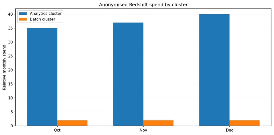
Almost all spend variability came from a single mixed-use analytics cluster.
The cost data also showed that the largest fluctuations were tied to compute and scaling behaviour, rather than storage growth. That shifted the focus toward runtime behaviour, CPU pressure, and scaling activity.
The working hypothesis was simple: the analytics cluster was relying on additional compute capacity for longer periods than expected.
Step 2: Start with cluster posture
Once we'd identified the cost-driving cluster, the next step was to review its posture.
The cluster used RA3 nodes, managed storage, Workload Management, and Concurrency Scaling. At a configuration level, nothing looked obviously broken. That is worth pausing on. A Redshift cluster can look reasonable from a static configuration view and still be poorly aligned with the way workloads actually use it.
The useful question wasn't is the cluster configured correctly? It was is the cluster configuration aligned with the workload pattern? That moved the investigation away from static configuration review and into runtime behaviour.
The cluster supported several workload types:
- BI dashboards
- Application-driven analytics
- Batch and transformation pipelines
- ML or campaign-related processing
- Scheduled data engineering jobs
This mixed-use pattern is common, but it needs careful workload isolation. Redshift Workload Management (WLM) defines query queues and routes work into those queues at runtime. AWS documents WLM as the mechanism for managing query queues, priorities, and workload routing.
When several workload types share one scaling-eligible queue, Concurrency Scaling stops being burst capacity.
Step 3: Let CloudWatch tell the story
The next step was to review a small set of CloudWatch metrics for Redshift.
The goal was to answer one question: was this cluster seeing short-lived bursts, or sustained pressure?
The most useful metrics were:
CPUUtilizationConcurrencyScalingActiveClustersConcurrencyScalingSecondsDatabaseConnections- Disk utilisation
The pattern became clear quickly.
Busy window: 00:00 to 09:00 UTC
This period had the strongest signs of pressure: highest CPU utilisation, highest database connection counts, most sustained Concurrency Scaling activity, and multiple workloads overlapping. That suggested batch, dashboard, and application workloads were colliding in the same time window.
Business-hours window: 09:00 to 17:00 UTC
Activity stayed elevated, although typically lower than the early window. This was likely driven by BI, dashboard usage, and interactive analytics.
Low-activity window: 17:00 to 23:00 UTC
This period showed more available headroom: lower CPU utilisation, reduced scaling activity, lower connection pressure. That made it a natural candidate for rescheduling lower-priority batch or transformation workloads.
Step 4: Concurrency Scaling was not behaving like burst capacity
The biggest finding was the Concurrency Scaling pattern. The cluster wasn't using Concurrency Scaling only during short spikes. It was using it for most of the day, often with multiple scaling clusters active at the same time. In the observed period, Concurrency Scaling was active for roughly 18 to 20 hours per day.
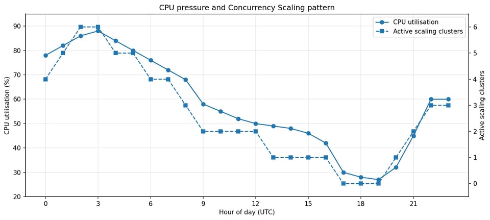
Concurrency Scaling tracked CPU pressure across most of the day, not just during spikes.
That changed the nature of the investigation. The question was no longer why did Redshift scale during a spike? It was why does this cluster need sustained overflow capacity?
Long-running Concurrency Scaling usage is a signal that the workload may be misaligned with baseline capacity, workload routing, or scheduling. At this point, the investigation shifted from "find the spike" to "understand the workload shape".
Step 5: Identify the bottleneck
The next step was to work out what was actually causing scaling pressure. There are several common possibilities:
- CPU saturation
- Queue wait time
- Disk pressure
- I/O pressure
- Connection pressure
- Poor workload routing
The metrics pointed strongly toward CPU. CPU utilisation stayed elevated, with frequent peaks during the same windows where Concurrency Scaling was active. Disk utilisation remained healthy. I/O and network throughput were active but didn't appear to be the primary bottleneck.
That matters because the fix for CPU saturation is different from the fix for queueing or storage pressure. Queue wait time points at WLM configuration and slot allocation. Storage pressure points at table design, data lifecycle, and managed storage usage. CPU pressure points at query efficiency, workload scheduling, queue isolation, and baseline compute capacity.
In this case, the cluster was doing a lot of work, for a long time, with many workloads competing for CPU.
Your cloud bill shouldn't be a mystery
Optimization, automation, expertise. In one platform.
Step 6: The WLM queue was the cost amplifier
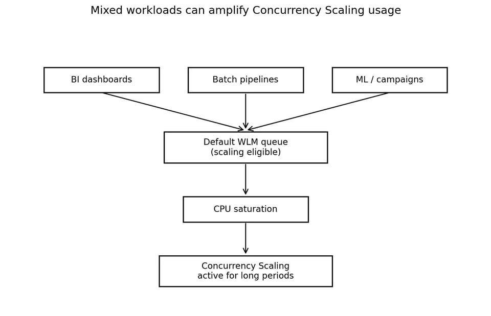
The next finding was in Workload Management. The configuration had multiple queues defined, but Concurrency Scaling was enabled on the Default Auto WLM queue, and that queue also acted as a catch-all for workloads not explicitly routed elsewhere.
This created a simple but expensive pattern:
Unclassified or mixed workloads vDefault Auto WLM queue (scaling enabled) vCPU pressure vConcurrency Scaling vHigher compute costThe issue wasn't that Auto WLM or Concurrency Scaling were "wrong". Both are useful Redshift features. The issue was that too much mixed workload was flowing through the one queue that had access to scaling capacity.
WLM routing can be based on user groups, query groups, and related classification rules, which makes it a key control point for workload isolation. If BI dashboards, batch jobs, ML workloads, and application queries all land in the same scaling-enabled queue, Concurrency Scaling becomes a broad escape hatch instead of a targeted tool.
That is how costs grow quietly.
Step 7: Connections are not the same as active concurrency
Another useful observation was around database connections. The cluster showed regular spikes in connection count, sometimes reaching high levels during busy windows. At first this looked like a possible connection limit problem.
But database connections are not the same thing as actively running queries. A Redshift cluster can have many established connections while only a subset of work executes at any given time, based on workload management, memory, CPU, and queue configuration. High connection counts are still a useful signal because they often indicate dashboard refreshes, application fan-out, or job bursts. They are not, by themselves, proof of active query concurrency.
In this investigation, the connection spikes were useful because they lined up with CPU pressure and Concurrency Scaling usage. That made them part of the story, not the root cause by themselves.
The better conclusion: many clients were connecting and submitting work during predictable windows, and the cluster didn't have enough effective compute headroom for that workload mix.
Step 8: Query visibility depends on database privileges
When investigating query behaviour, Redshift system tables and views are essential. One common point of confusion is query visibility. In Redshift system views, superusers see all rows, while regular users generally see only their own data. AWS notes this visibility rule for views such as SYS_QUERY_HISTORY, STL_WLM_QUERY, STL_QUERY_METRICS, and related monitoring views.
For cluster-wide workload analysis, the person running the queries needs the right database permissions.
Useful questions to answer include:
- Which users consume the most execution time?
- Which queries run during the busy window?
- Which workloads use Concurrency Scaling?
- Which queues receive most of the work?
- Which queries repeat frequently enough to be worth optimising?
Where available, AWS recommends the newer SYS monitoring views because they are formatted to be easier to use and understand. The older STL and SVL views are still widely used and useful for investigations, but the SYS views are a cleaner starting point when they cover what you need.
Top queries by execution time
SELECT h.user_id, u.usename AS user_name, h.query_id, h.query_type, h.status, h.start_time, h.end_time, h.elapsed_time / 1000000.0 AS elapsed_seconds, h.execution_time / 1000000.0 AS execution_seconds, h.queue_time / 1000000.0 AS queue_seconds, h.service_class_name, h.compute_type, LEFT(h.query_text, 500) AS query_text_sampleFROM sys_query_history hLEFT JOIN pg_user u ON h.user_id = u.usesysidWHERE h.start_time >= dateadd(day, -7, current_date)ORDER BY h.execution_time DESCLIMIT 50;Top users by total execution time
SELECT h.user_id, COALESCE(u.usename, 'unknown') AS user_name, COUNT(*) AS query_count, SUM(h.execution_time) / 1000000.0 AS total_execution_seconds, SUM(h.queue_time) / 1000000.0 AS total_queue_secondsFROM sys_query_history hLEFT JOIN pg_user u ON h.user_id = u.usesysidWHERE h.start_time >= dateadd(day, -7, current_date)GROUP BY h.user_id, u.usenameORDER BY total_execution_seconds DESC;Top queries by CPU time
SVL_QUERY_METRICS_SUMMARY is useful here because it includes query_cpu_time, query_blocks_read, and related metrics for completed queries. AWS documents query_cpu_time as CPU time used by the query, in seconds.
SELECT h.user_id, COALESCE(u.usename, 'unknown') AS user_name, h.query_id, h.start_time, h.service_class_name, h.compute_type, m.query_cpu_time, m.query_execution_time, m.query_blocks_read, m.query_temp_blocks_to_disk, LEFT(h.query_text, 500) AS query_text_sampleFROM sys_query_history hJOIN svl_query_metrics_summary m ON h.query_id = m.queryLEFT JOIN pg_user u ON h.user_id = u.usesysidWHERE h.start_time >= dateadd(day, -7, current_date)ORDER BY m.query_cpu_time DESCLIMIT 50;WLM queue usage
SELECT service_class_name, compute_type, COUNT(*) AS query_count, SUM(queue_time) / 1000000.0 AS total_queue_seconds, SUM(execution_time) / 1000000.0 AS total_execution_seconds, AVG(queue_time) / 1000000.0 AS avg_queue_seconds, AVG(execution_time) / 1000000.0 AS avg_execution_secondsFROM sys_query_historyWHERE start_time >= dateadd(day, -7, current_date)GROUP BY service_class_name, compute_typeORDER BY total_execution_seconds DESC;Queries that ran on Concurrency Scaling
In SYS_QUERY_HISTORY, the compute_type column identifies whether a query ran on the main cluster or a Concurrency Scaling cluster for provisioned Redshift clusters. AWS documents primary-scale as the compute type for a query that runs on a concurrency cluster.
SELECT h.user_id, COALESCE(u.usename, 'unknown') AS user_name, h.query_id, h.start_time, h.end_time, h.execution_time / 1000000.0 AS execution_seconds, h.service_class_name, h.compute_type, LEFT(h.query_text, 500) AS query_text_sampleFROM sys_query_history hLEFT JOIN pg_user u ON h.user_id = u.usesysidWHERE h.start_time >= dateadd(day, -7, current_date) AND h.compute_type = 'primary-scale'ORDER BY h.start_time DESCLIMIT 100;These queries are not the end of optimisation. They are the start of prioritisation. The point is to stop guessing and identify which workloads should be isolated, rescheduled, tuned, or allowed to use scaling.
Step 9: Recommended remediation plan
Once the pattern was clear, the remediation plan became straightforward. The goal wasn't to switch Concurrency Scaling off blindly. That would likely reduce cost, but it could also increase queueing and slow down important workloads.
A safer approach is phased, starting with low-risk routing changes and moving toward decisions that cost more to reverse.
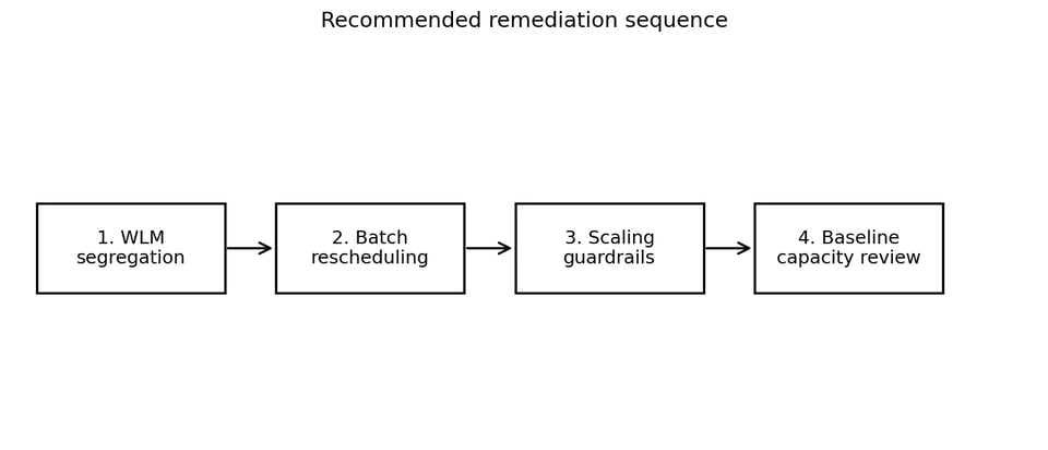
A phased order keeps the early steps cheap and reversible.
1. Segregate workloads with WLM
WLM should reflect workload priority. For example:
| Workload type | Possible treatment |
|---|---|
| BI dashboards | Higher priority, limited scaling access |
| Critical application queries | Higher priority, protected queue |
| Batch jobs | Dedicated queue, often no scaling |
| ML or transformation workloads | Dedicated queue, scheduled where possible |
| Ad hoc analysis | Lower priority or restricted scaling |
This prevents lower-priority batch work from consuming the same scaling pool as interactive or business-critical queries. It's a routing change, so it can be rolled back quickly if a queue boundary is wrong.
2. Move batch jobs into low-activity windows
The metrics showed a clear low-activity window later in the day, which creates an immediate operational lever.
Not every batch job needs to run during the busiest period. Moving lower-priority transformation, ML, or reporting jobs into quieter windows can reduce peak CPU pressure without changing cluster size. This is often one of the most practical cost levers because it changes timing, not architecture.
3. Add Concurrency Scaling guardrails
With workloads correctly routed and timed, the next step is to cap Concurrency Scaling itself. If it's allowed to scale too broadly, it can protect performance but create unpredictable cost.
A reasonable first step is to reduce the maximum number of allowed scaling clusters to a controlled level, then observe the impact. That helps answer:
- Which workloads begin to wait?
- Which jobs are truly latency-sensitive?
- Which workloads were relying on scaling capacity without a business reason?
The point isn't to degrade performance. It's to make scaling an intentional resource, not an unlimited default.
4. Revisit baseline capacity
If Concurrency Scaling remains active for long periods after WLM and scheduling changes, the baseline cluster may simply be under-sized for the workload. In that case, adding base capacity can be cheaper than continuously relying on overflow capacity.
This is counter-intuitive but common: increasing baseline capacity can reduce total cost if it materially reduces sustained Concurrency Scaling usage.
The key is to make this decision after workload isolation and scheduling have been improved. Otherwise you risk adding nodes while still allowing inefficient workload routing to consume scaling capacity.
5. Tune queries with evidence
Query optimisation should focus on the workloads that matter most:
- High total execution time
- High CPU consumption
- Frequent repeated execution
- Execution during busy windows
- Queries that land in scaling-enabled queues
This is where the system table analysis becomes useful. Optimise the queries that materially affect cost and performance, not the queries that just look ugly.
Key takeaways
This investigation reinforced a few practical Redshift lessons.
Concurrency Scaling shouldn't become baseline capacity. If it's active for most of the day, it's no longer behaving like burst capacity. It has become part of the steady-state compute model, and that's a cost signal.
CPU pressure and queue pressure are different problems. High Concurrency Scaling usage doesn't automatically mean WLM queueing is the root cause. Check CPU, queue wait time, disk, I/O, and connection patterns together.
Default queue routing can be expensive. A catch-all queue with Concurrency Scaling enabled can quietly become the main cost amplifier. WLM routing should match workload priority.
Workload timing matters. If batch jobs, dashboards, ML workloads, and application analytics overlap, scaling pressure increases. Moving non-critical batch workloads to quieter windows can reduce cost without changing functionality.
Query tuning should follow attribution. Before tuning queries, identify which users, workloads, and queues are driving resource consumption. Guessing usually wastes time.
Closing thoughts
Redshift cost optimisation is rarely about one setting. In this case the issue wasn't a broken cluster or a single bad query. It was a combination of mixed workloads, predictable timing collisions, CPU saturation, and broad access to Concurrency Scaling through the default WLM path.
The most useful part of the investigation wasn't any single metric. It was connecting them:
- Cost report identifies the cluster
- CloudWatch shows sustained scaling and CPU pressure
- WLM configuration explains why scaling is broadly available
- System tables identify which users and queries to prioritise
If your Redshift bill is climbing and Concurrency Scaling has quietly drifted from burst to baseline, you're not alone. This is the kind of cost investigation DoiT runs with AWS customers every week. Our team of 100+ cloud experts can help you spot the drivers, segregate workloads, and put Concurrency Scaling back where it belongs. Get in touch.