Photo by eMotion Tech on Unsplash

Preface

The following blog will introduce a way of tackling a known challenge in data warehouse systems of keeping fresh and updated data but avoiding large mutations.
At DoIT, we work with many customers on building well-architected systems, using cloud services efficiently, and the following is derived from a customer story.

Background

A SaaS company offers its customers an analytical platform on top of BigQuery. For some customers, the data is received as a complete snapshot, including the full history and not only the incremental changes from the last update.
One of these customers provides a snapshot of 15TB, while the actual updated data is only 0.1%. As there was no way to acquire only the incremental changes update, the team had the challenge of finding the most reliable and efficient manner in performance and cost of keeping the existing table updated with new snapshot data.

Data pipeline requirements

The company and the customer defined a data contract for the data pipeline to fulfill the business and technical requirements:

• Incoming Data is a complete snapshot of a two-year sliding window, and its arrival cadence is six times daily.
• The data is partitioned by day (partition size is about 20GiB~ and is marked with a snapshot ID (an incremental value).
• Data will contain new data (new keys) and changed data (updates to existing data).
• Partition expiration configuration to 2 years.
• Records in the current snapshot but missing in the new snapshot will remain until partition expiration.

The SaaS company product team defined the following requirements:

• Modeling: Two tables will contain the existing and new data.

New data resides in a table named “staging”, and existing data (data exposed to the customer) lives in a table called “target”.

• Uniqueness: The “target” table data is unique (no duplicate keys).
• Freshness: The ‘’target” table will refresh within one hour from the arrival of the snapshot.
• Availability: The end user always gets a response to a query request.

 

The Mutation Challenge:

As the following Google Blog describes, BigQuery isn’t built like OLTP transactional processing DB’s that are natively efficient in significant mutations.

“BigQuery is not unique among OLAP databases in being constrained on mutation frequency, either explicitly (through quotas) or implicitly (resulting in significant performance degradation), since these types of databases are optimized for large-scale ingestion and analytical queries as opposed to transaction processing. Furthermore, BigQuery allows you to read the state of a table at any instant in time during the preceding seven days. This look-back window requires retaining data that the user has already deleted. To support cost-effective and efficient queries at scale, BigQuery limits the frequency of mutations using quotas.” (Performing large-scale mutations in BigQuery | Google Cloud Blog )

A complete replacement that removes and replaces the old snapshot with the new snapshot isn’t sufficient, as there is a need to keep records that exist in the current snapshot but are missing in the latest snapshot.
It means there is a need to compare records between the existing and new snapshots, while the regular replacement approach won’t make such a comparison.

To show the mutation options and their differences, let’s define the problem precisely with the exact data modeling and mutation logic.

Data modeling

Table Schema:

A record in a table (‘staging’ or ‘target’) contains an attribute_id and value for a specific product (product_id) in a store (store_id) for a particular date and the reference for the snapshot it existed (update_id).

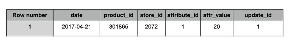
Record example:
Based on data received in snapshot ID 1 (update_id), the Total quantity value (attribute_id = 1) of a product (product_id = 301865) in a store (store_id = 2072) was 20 on 2017–04–21.

Mutation logic example:

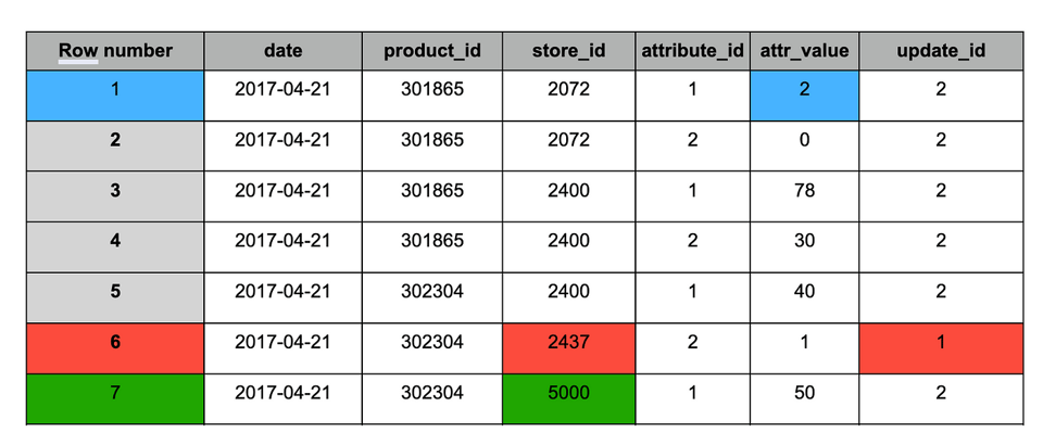
The following is an example of a sample from one partition (specific date) from two different snapshots.

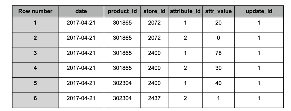
target’ table after ingestion of snapshot #1

Snapshot #2 contained the following changes:

1. Blue: updated records (appears in both snapshots), value changed.
2. Red: historical record (appears only in snapshot #1).
3. Green — new record (appears only in snapshot #2).

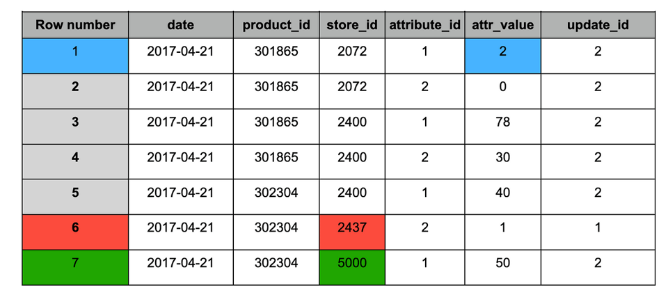
target’ table after ingestion of snapshot #2

As BigQuery supports MERGE, merging the staging table with the target table is the intuitive approach, using the following logic.

Merge logic:

This MERGELogic defines the mutations to be applied according to the different cases based on a joined key specified by the following fields: product_id,store_id,attribute_id

This is the code implementation of the MERGElogic:

MERGE
nw-playground.demo.merge_target T
USING
nw-playground.demo.merge_staging S
ON
 T.product_Id = S.product_Id
 AND T.store_Id = S.store_Id
 AND T.attribute_Id = S.attribute_Id
 AND T.date = S.date
 WHEN MATCHED and T.date  >= '2017-04-14' and T.date <= '2017-04-26'
 THEN UPDATE SET T.attr_value = S.attr_value, T.update_id = S.update_id
 WHEN NOT MATCHED BY TARGET  and S.date >= '2017-04-14' and S.date <= '2017-04-26'
 THEN
INSERT
 (date,
   product_Id,
   store_Id,
   attribute_Id,
   attr_value,
   update_id)
VALUES
 (S.date, S.Product_id, S.store_Id, S.attribute_Id, S.attr_value, S.update_id);

Problem:

As mentioned above, the MERGEoperation is very costly in BQ and has limitations, requiring shuffling and mutation of the existing data.

So, we need to Find a way to avoid the MERGE and data mutation.

Deduplicate and Clone approach:

What will we do?
Instead of merging the ‘staging’ and ‘target’ table records, we’ll perform the following steps:

1. Append the new snapshot to the ‘staging’ table.
2. Deduplicate similar records and keep the newest record.
   
   Deduplication is a process used to remove duplicated records and leave only a single record. Deduplication is achieved by setting a record key to identifying similar records and logic to decide which to keep between the duplicated records (i.e., the newest record.)
3. Replace the ‘staging’ table with the deduplication results.
4. Replace the ‘target’ table with a CLONE of the ‘staging’ table.

“CLONEA table clone is a lightweight, writeable copy of another table (called the base table). You are only charged for data storage in the table clone that differs from the base table, so initially, there is no storage cost for a table clone. Other than the billing model for storage and some additional metadata for the base table, a table clone is similar to a standard table — you can query it, make a copy of it, delete it, and so on. After you create a table clone, it is independent of the base table. Any changes made to the base table or table clone aren’t reflected in the other.” table-clones-intro

How will we do it?

1. Data appending: using the LOADcommand in ‘append’ mode so the staging table will have the current and the new snapshot.
2. Deduplication: deduplicate similar records (same key) and keep the newest record between them. The deduplication does not impact records that are entirely new or exist only in the current snapshot. Deduplication is implemented using ‘Windows functions’ that compute values over a group of rows and the QUALIFYoperation. The QUALIFYclause can filter the results of a window function (group of rows).
3. Replace ‘staging’: using the CREATE OR REPLACEbased on the deduplication query results
4. Clone ‘staging’ to ‘target’: using CREATE OR REPLACE TABLE ... CLONE

Why do we do it?

This benefits from a few aspects in conjunction with the MERGEapproach:
1. Reduce data shuffling: Appending the new snapshot to the existing one avoids shuffling between two tables.
2. Avoid MERGE/JOINoperation: deduplication is implemented by a window function that uses the PARTITION BYclause, which breaks up the input rows into separate partitions, over which the window function is independently evaluated.
3. Avoid mutation: new tables are created or cloned. Avoids BigQuery mutation quota limits.

Example of appending and deduplication logic:

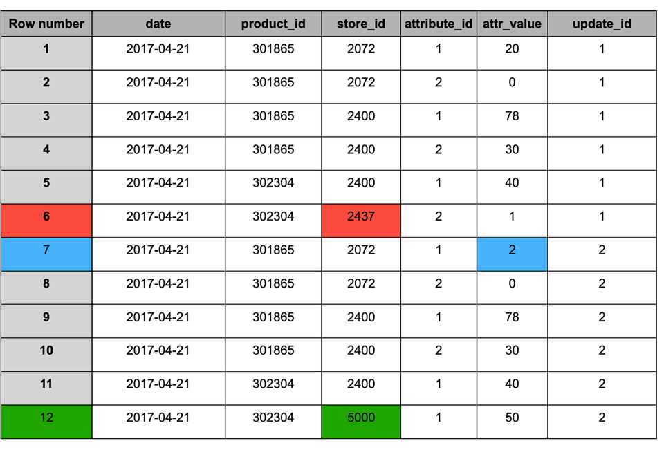
Staging table after appending the new snapshot (#2)

Similar to the MERGEresult, the table after deduplication contains the following changes:
1. Blue — updated records (appears in both snapshots), the value changed.
2. Red — old records that should be kept (appears only in snapshot #1).
3. Green — new record (appears only in snapshot #2).

Staging table after deduplication

When the next snapshot arrives, it will follow the same process as above.

Code examples:

The following code creates a new staging table from the deduplication results that replaces the existing table by using theQUALIFY clause and adding a row number to each record with a similar key, while the 1st record (rownum=1) is the newest.

CREATE OR REPLACE TABLE
 `nw-playground.demo.dedup_staging` 
 (date DATE,    product_id INT64,
  store_id INT64,    attribute_id INT64,
  attr_value INT64,    update_id INT64)
PARTITION BY
 date
CLUSTER BY
 product_id,
 store_id AS
SELECT
 date,  product_id,  store_id,  attribute_id,  attr_value,  update_id
FROM
 `nw-playground.demo.dedup_staging`
WHERE
 date >= '2017-04-14' AND date <= '2017-04-26'
 QUALIFY ROW_NUMBER() 
 OVER(PARTITION BY date, product_id, store_id, attribute_id
 ORDER BY update_id DESC ) = 1;


CREATE OR REPLACE TABLE
`nw-playground.nw_demo.dedup_target`
CLONE `nw-playground.nw_demo.dedup_staging`;

Testing data and results:

Testing has been done on 7.8 Billion records (350GiB) distributed to 13 partitions with 3M~ differences (all types of changes), between the ‘staging’ and ‘target’. Tests were performed using on-demand billing model.

In the MERGEcase, the ‘staging’ table contained only the new snapshot, and the ‘target’ table had the existing snapshot. In contrast, in the deduplication case, the staging table had the existing and new snapshots and the ‘target’ was a clone of the staging 1st snapshot.

Results comparison:

The following table shows the comparison of the results:

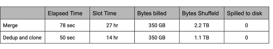
Execution details summary comparison

Comparing the execution plans, it’s clearly shown that the duration and slots utilization of the MERGEthe test is double that in the DEDUPLICATE:

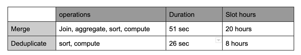
Main operation duration and slot utilization

Cost Comparison

On-demand billing model:

The cost is similar between tests as we scan the same data size. It will reach around 187$ (6.25$ for 1TiB) in full load, based on 30TB 2 snapshots.

BigQuery Editions:

The new billing model introduced by Google on APR/23 is based on capacity pricing (pay per slot/hour) and has three editions. To calculate the cost for production load, we can estimate a full snapshot load in a factor of 56 compared to the test we’ve done (730 days-partitions in 2 years, 730/13=56.
The cost estimation isn’t accurate as there are also different configurations and commitments to be applied. It mainly shows the difference between the two options.

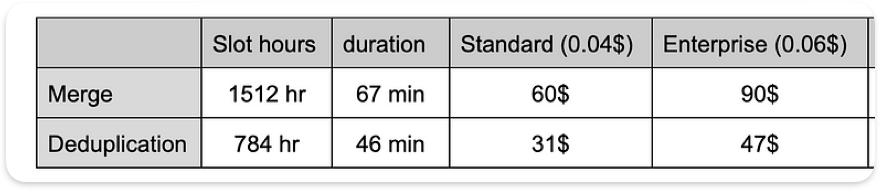
Compare estimation cost between BigQuery editions (US pricing)

Summary

As described in the use case, a large-scale mutation is involved, which relies on a join logic with the existing data. The preferred way to tackle it is by avoiding modifications to the data.
Using the ‘deduplication’ and CLONE option avoids DML limitations and significantly improves both dimensions, Elapsed Time and Slot utilization, resulting in a 50%~ performance and cost reduction.

Appendix

There are several ways to implement deduplication (using ROWNUM or Group By). Trying deduplication using ROWNUM has performed similarly to the QUALIFY clause. Hence, QUALIFY is a cleaner command. Using “Group By” resulted in worse performance, identical to Merge results.

There can be another efficient way of implementing: stored procedures for Apache Spark, to be continued in the next Blog…