As some of you might already know, DoiT International is the engineering power behind reOptimize — Cost Discovery and Optimization SaaS for Google Cloud Platform.
With reOptimize you can get instant insights on your Google Cloud Platform billing, manage budgets, set up cost allocations and explore different cost optimization strategies.
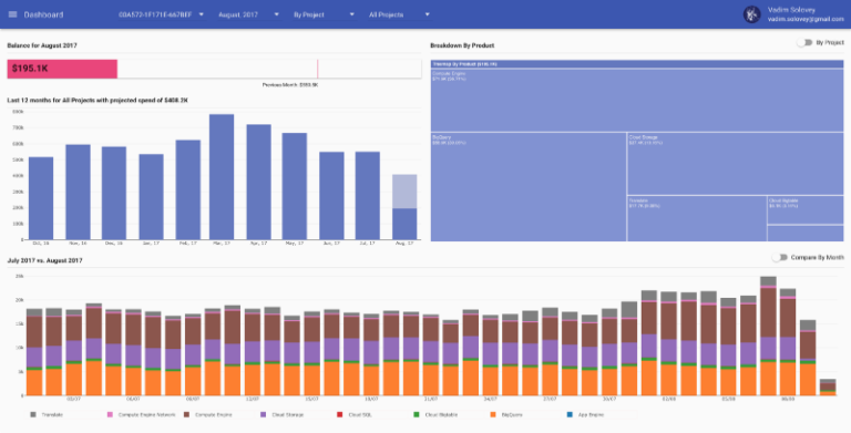
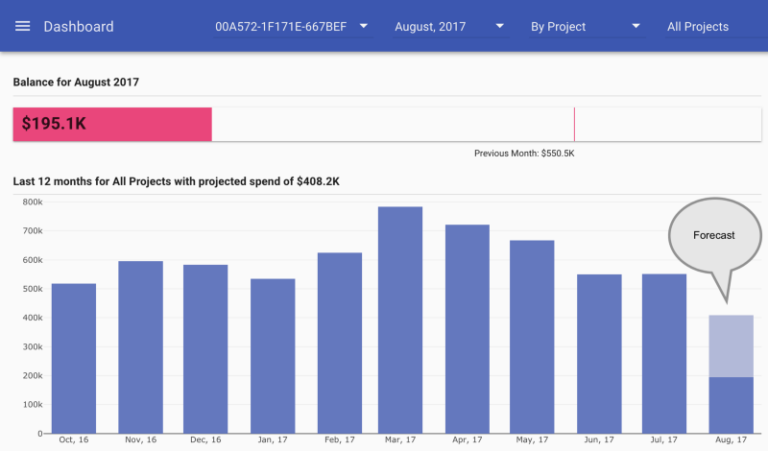
One of the features we had from the day one is an estimation on how your monthly bill will look like at the end of the month. Here is how it looks like in reOptimize’s dashboard:
Initially, our estimation model used a very trivial linear regression — taking the current spending and the day of the month and extrapolating the value assuming spending will increase linearly. We did make some adjustments such as taking into consideration Google Compute Engine Sustained Discounts and few other things as well but still it was very naive and simplistic.
Unfortunately cloud services are cumulative, and in general, the cloud spending by itself doesn’t act linearly at all. There are seasonality patterns such as longer or shorter months, holidays seasons, marketing campaigns and so much more! The estimation given by this model usually is pretty far off. We calculated it to have a root-mean-square deviation (RMSE) of ~900.
Since many of our customers rely on reOptimize to forecast their Google Cloud Platform spendings, we started to work on Machine Learning based model to increase the accuracy of our estimations.
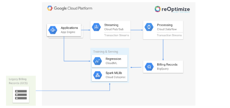
Naturally, we decided to use TensorFlow —an open-source software library for Machine Intelligence and specifically the Google CloudML which is Google’s managed service for TensorFlow so we would not need to take care of scaling, deployment, monitoring and other not too fascinating operational burden ;-)
There are three major parts to a our project:
- Preparing the historical data in order to train our model
- Training a prediction model
- Deploying the model to be used by reOptimize
All of these need to be automatically performed iteratively as new billing data arrives daily.
Preparing Training Data
Google Cloud Billing API can export billing records into a variety of destinations and one of these is Google BigQuery. We are using BigQuery table as a source of data to train our prediction model.
The information in the table has the following columns:
project.id - The GCP project ID
product - The GCP service name (i.e. BigQuery, Compute Engine, etc.)
start_time - The date and time of this billing row
cost - The Cost in US Dollars
credits.name - A repeated field with names of relevant credits
credits.amount - A repeated field with amount of relevant credits
To optimize the training process, we want to transform the raw data into a format better suitable for TensorFlow. This includes both the format and the semantics of the data.
TensorFlow supports multiple formats but the standard format is called TFRecords format. There are many built-in utilities to read and write data in this format.
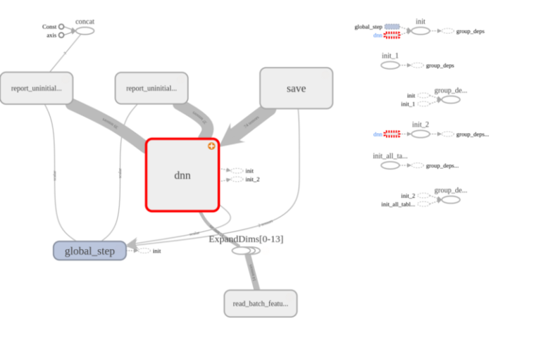
The data semantics itself should be transformed into values best fitted for a DNN. The DNN or a Deep Neural Network — is a type of mathematical model that is used in machine learning and is built on the basis of the functionality of a human brain.
A DNN doesn’t work well with inputs that are not numbers and preferably numbers with real meaning. For example, product names and project names do not really mean anything on their own as well as year values and month values. On the other hand, the day numeric value has such meaning as well as the cost. Also feeding the raw cost rows would not be productive as we need to supply a target value per sample.
We are transforming the data from BiqQuery into something better suited for our DNN model.
The way we thought would be best to define our samples is to create a daily aggregation for a product and project and the sum of the costs from the beginning of the month up to that day. We also need to add the total cost for that product and project at this month and use that as the target value to train on. Finally, the product and project names must be first mapped into integers.
In our case, each sample would include the project, product, day, partial cost (from beginning of month) and total cost. In order for the DNN to be able to understand the data we want to augment the sample with additional data that mind prove useful but hard for the DNN to calculate on it’s own.
The number of days in the current month is an arbitrary constant that may affect the total cost. We can “calculate” this for the DNN, thus saving time and complexity. We can also calculate the ratio of cost per day by dividing the partial cost from the current day.
Another useful value would be the mean ratio and mean total cost for the product and project — these values would probably be used by a humans when trying to forecast the monthly bill. We can easily get BigQuery to build us a mapping table that provides these mean values per project and product and we used this table to create a static lookup table to enrich samples with.
Some other ratios were also calculated to provide more information for the DNN to use such as the estimated linear total cost (i.e. ratio * days in month)
Now that we have the data, we would feed the samples, one by one, along with the label value for the sample. We will train the model to predict the total cost from the sample input values. This way we could later use the model to feed the current spending and date per project and product and predict the total cost for the end of the month.
Now that we have our data ready, we wanted to have a way to evaluate our model against what we have today. We used the transformed data to calculate the simple linear regression performed by our code today. Each sample was calculated and then we subtracted the expected total from the prediction, squared the value and then calculated an average for this value for all samples. The square root of this value is the RMSE. We got an RMSE of ~900.
Looking at the data at this stage it was obvious that it didn’t behave in any linear fashion. Trying to create a DNN that would predict such data would be very hard — but we can help build a simpler DNN by feeding the network with some calculated values which we already know are relevant. To do that we would like to enrich the data as well as transform it.
One thing that looks helpful is to feed a value with the ratio between the current cost from start of month and the days since start of month. This value can also be averaged over each month and even globally to provide some more relevant info about spending behaviour.
And of course, it might help the DNN to know the history of total cost for previous month so we add the average total cost over each month and also a global average of the total cost.
This is the preprocessing function we built:
We then want to package it all together in TFRecord format ready to be trained. Luckily a package already exists that can help us to it. The python tensorflow-transform package uses a combination of Tensorflow and Apache Beam to process large amounts of data, transform them and write them into TFRecord files.
Another advantage of tensorflow-transform is that it creates a TensorFlow graph to process the data and runs it through a Beam pipeline — and that means you can use this graph later for the prediction — thus doing all these transformations on the data for you so you don’t need to transform the data prior to feeding it for prediction.
At the heart of the preprocessing script we run the Apache Beam pipeline:
The get_data_from_bq function reads the BigQuery data by using the SQL query shown above.
It then uses AnalyzeAndTransformDataset to perform the processing itself. The AnalyzeAndTransformDataset needs a pre-processing function to define the transformation graph. The transformed data is written using TFRecord formats into two file sets for training and testing.
In addition to the data, the pipeline also saves the metadata for the model, including the raw input metadata, the transformed data metadata and the transformation function graph. These are later used for training the model.
Training the Model
After the data is ready, the next step is to train a model with the data we have just prepared.
We decided to use a simple DNN and train it using the TensorFlow DNNRegressor class. The metadata created by tensorflow-transform in the pre-processing step is now used to create input functions for training, testing and serving.
Finally we use TensorFlow contrib.learn.Experiment to coordinate the training and evaluation.
To do this we define a function which generates the experiment:
And then use it to run the experiment:
The result of this process is a folder with the saved model which we can later deploy to Google CloudML to do actual predictions.
Deploying the Model
To allow reOptimize use the predictions, we obviously need to create some infrastructure that serves API requests coming from the application returning the output from the model.
Google CloudML does exactly that with TensorFlow Serving. TensorFlow Serving uses a trained model saved into a local disk or a GCS bucket to run the model and retrieve output. It exposes a RESTful API that can be used by any web or mobile client. Google CloudML takes it a step further by providing a serverless, fully managed serving infrastructure for your model so you don’t need to set up machines, autoscale them and so on..
After our model has been trained and saved, we are deploying it using the gcloud command line.
$ gcloud ml-engine models create reoptimize --regions=us-east1
$ gsutil -m cp -r job/model/export/Servo/... <MY_GCS_BUCKET_NAME>/model/<MODEL_VERSION_NAME>
$ gcloud ml-engine versions create <MODEL_VERSION_NAME> --model reoptimize --runtime-version 1.2 --origin <MY_GCS_BUCKET_NAME>/model/<MODEL_VERSION_NAME>
$ gcloud ml-engine versions set-default <MODEL_VERSION_NAME> --model reoptimize
This will create a URL that can be used to predict using our model. The URL points to a fully managed backend API service created by Google CloudML.
It can both handle REST calls as well as be used by the gcloud command line tool like this:
gcloud ml-engine predict --format=json --model reoptimize --json-instances=data/predict.json
The data/predict.json file contains information such as this:
And the results would be something like this:
Summary
By implementing machine learning to predict Google Cloud Platform bills, our forecast are now much more accurate. They are taking (indirectly) into account huge amount of signals such as seasonality, changes in pricing models, marketing campaigns and so on.
Our RMSE went down from ~900 to just ~100 so our predictions are much more credible and can be relied on by our customers.
By using Google CloudML, Dataflow and BigQuery, we could implement the machine learning infrastructure in reOptimize in just couple of weeks, while investing more time into the engineering rather than operations or maintenance.