
How to save time and money processing your BigQuery queries
Part of the process of spending less to achieve more with BigQuery is to recognize some of the common mistakes people make when writing BigQuery queries. If you want to speed up your query processing and reduce the costs involved, you should avoid eight common mistakes:
1. SELECT *
SELECT * is probably the biggest source of unnecessary additional costs with BigQuery queries.
When you select all the columns in a table or view, you’re usually simply scanning excess data. You may have to do a SELECT * in a few cases, including when you have filtered down a view already, used a Common-Table-Expression (CTE) to reduce the data needed or you have a small table where all of the data in it is needed (such as a fact table).
Otherwise, performing a SELECT * on your data simply increases your BigQuery bill because BigQuery bills are based on the volume of data you scan in your queries when on an on-demand pricing model.
For example, if you perform a SELECT *on a 5TB table with five columns containing equal volumes of data, all of which has to be scanned, that query will cost $25, whereas a query involving a SELECT * only on the two columns you need would cost just $10. The costs quickly add up for queries run multiple times a day.
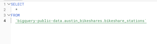
Example of using a SELECT * on a very large public dataset query
2. Unnecessary or larger joins
For data warehouses that focus on an OLAP strategy (like BigQuery), you are advised to denormalize the schemas in the database to flatten the data structures and minimize the number of joins required versus a traditional relational database. This is because a join operation is much slower within BigQuery than it is for a traditional database, due to the way the data is stored in the underlying system. Joining large tables obviously takes more time and scans more data than simply storing the required data (or a copy) in the same table.
You should also avoid the “self-join,” where data from the table might need to be broken up into windows of time or to put an internal ordering on duplicate rows (called ranking in many database systems). This is exceedingly slow, so use the window or analytic functions provided by BigQuery instead.
Here is an example of ranking duplicate job IDs in your INFORMATION_SCHEMA view:
SELECT
 query,
 job_id AS jobId,
 COALESCE(total_bytes_billed, 0) AS totalBytesBilled,
 ROW_NUMBER() OVER(PARTITION BY job_id ORDER BY end_time DESC) AS _rnk
FROM
 `<project-name>`.`<dataset-region>`.INFORMATION_SCHEMA.JOBS_BY_PROJECT
3. Cross joins
Cross joins are not something anyone from a Relational Database Management System (RDBMS) with a software engineering background would use, but they are required for several things in BigQuery. The principal use case is unnesting arrays into rows – a fairly common operation when working on analytical data.
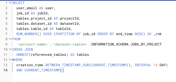
Example of unnesting a RECORD typed column using a CROSS JOIN
However, if you use cross joins as the innermost operation in your query, they pull in far more data than will be passed to the output, prompting BigQuery to bill you to scan and read a lot of data that may be thrown away at a later phase in the query. Instead, perform your cross joins at the outermost possible point in your query to minimize the volume of data being read before doing the cross join. This reduces your slot count and the volume of data you have to pay for.
4. Using Common Table Expressions (CTEs) incorrectly
Common Table Expressions (CTEs) are wonderful for breaking up SQL code that’s getting deep into multiple levels of subqueries. Generally used for readability rather than performance, they do not materialize the data and will be rerun if used multiple times. The biggest cost and performance issue I see is using a CTE in a query while referencing it multiple times. The CTE query is then run multiple times, so you will be billed for reading the data multiple times.
5. Not using partitions in WHERE clauses
Although partitions are one of the most important features of BigQuery for reducing costs and optimizing read performance, they are frequently omitted, incurring unnecessary spending on queries. A partition breaks up a table on disk into different physical partitions, based on an integer or timestamp/datetime/date value in a specific column, so when you read data from a partitioned table and specify a range on that column, it only needs to scan over the partitions that contain the data in that range – not the whole table.
The following query pulls the total billed bytes for all queries in the past 14 days. The JOBS_BY_PROJECT is partitioned by the creation_time column (schema doc is here) and, when run against a sample table with a total size of about 17GB, it processes 884 MB of data.
DECLARE interval_in_days INT64 DEFAULT 14;

SELECT
 query,
 total_bytes_billed AS totalBytesBilled
FROM
 `<project-name>`.`<dataset-region>`.INFORMATION_SCHEMA.JOBS_BY_PROJECT
WHERE
 creation_time BETWEEN TIMESTAMP_SUB(CURRENT_TIMESTAMP(), INTERVAL interval_in_days DAY)
   AND CURRENT_TIMESTAMP()
The following query is run using the start_time column, which is not partitioned but usually within fractions of a second close to the creation_time value, against a sample dataset it processes 15 GB of data. The logic is that it scans the whole table pulling the requested values out.
DECLARE interval_in_days INT64 DEFAULT 14;

SELECT
 query,
 total_bytes_billed AS totalBytesBilled
FROM
  `<project-name>`.`<dataset-region>`.INFORMATION_SCHEMA.JOBS_BY_PROJECT
WHERE
 start_time BETWEEN TIMESTAMP_SUB(CURRENT_TIMESTAMP(), INTERVAL interval_in_days DAY)
   AND CURRENT_TIMESTAMP()
The contrast is stark, even on a smaller dataset: Given that the first query costs about $0.004 and the second about $0.75, failing to use a partitioned column properly is roughly 21 times more expensive.
Performance is also an issue, with the first query taking about two seconds to run and the second about five. Scaling up to a multi-TB table could easily generate multiple-minute differences per query run.
6. Using overcomplicated views
As with most of its pseudo- and real-relational brethren, BigQuery supports a construct called a view. Essentially, a view is a query that masquerades its results as a table for easier querying. If the view contains very heavy computations that are executed each time the view is queried, it can degrade the query’s performance substantially. If the logic in a view is excessively complicated, it might be better suited to pre-calculation into another table or living in a materialized view to enhance performance.
7. Small inserts
BigQuery is best for processing substantial chunks of data at a time, but sometimes it’s necessary to insert a small number of records into a table, especially in some streaming types of applications.
For small inserts, inserting 1KB or 10MB generally takes similar amounts of time and slot usage. Doing 1,000 inserts of a 1KB row could take up to 1,000 times as much slot consumption time as a single insert of 10MB of rows. Rather than doing multiple small inserts, batch up data and insert it as a batch. The same is true for streaming operations: Instead of using Streaming inserts, batch up your data before inserting it with a deadline for arrival.
8. Overusing DML Statements
This is a big issue that usually arises when someone approaches BigQuery as a traditional RDBMS system and simply recreates data at will.
These are three relatively common examples:
DELETE TABLE <table-name> IF EXISTS;
CREATE TABLE <table-name> ...;
INSERT INTO <table-name> (<columns>) VALUES (<values>);
TRUNCATE TABLE <table-name>;
INSERT INTO <table-name> (<columns>) VALUES (<values>);
DELETE FROM TABLE <table-name> WHERE <condition>;
INSERT INTO <table-name> (<columns>) VALUES (<values>);
Although running these on an RDBMS such as SQL Server or MySQL would be a relatively inexpensive operation, they perform very poorly within BigQuery. It is not optimized for doing DML statements in the same way that a traditional RDBMS is, so consider using an “additive model,” instead. In this model, new rows are inserted with a timestamp to indicate the latest, and older rows are deleted periodically if history is not needed.
BigQuery is a data warehouse tuned for analytics, so it’s designed for working with existing data rather than modifying data in a transactional manner.
What to do next
This article is condensed from my series of articles on optimizing your BigQuery queries.
At DoiT, we have deep, broad expertise in BigQuery and across the areas of machine learning and business intelligence. To avail of our support, get in touch.