Primer on BigQuery Cost and Performance Optimizations

Other parts in this series:
Part 1
Part 3

Continuing On

In the first part of this series I outlined some prerequisite knowledge and some operational items that need to be done in order to run queries and do the process of optimization.

In this part of the series I am going to cover the most common querying mistakes that end up costing our customers more money or cause performance issues. Consider this a primer for referring to later on ways to fix what you find in the later parts of the series.

If you are thirsting to do some “doing” on the optimizations go ahead and jump to part 3 of this series where I will give some queries then cover how to use them.

Common Query Mistakes that Cause Cost and Complexity Increases

Before I jump into the queries that will give you the actual data I want to give some examples of very common mistakes we see in writing BigQuery queries that can cause queries to take longer than needed to process and almost all of the time also cost more money.

These are all documented online, but I want to put in the most common ones that we see here at DoiT International working with hundreds of customers on a regular basis.

SELECT *

This is probably the largest cause of extra costs both in money spent and quantity of customers that do it.

There are some scenarios where you will need to select all of the columns in a table or view, but most of the time it’s unnecessary and is just scanning excess data. These scenarios are usually when you have already filtered down the scope of a view or used a Common-Table-Expression (CTE) to the data needed or you have a small table, such as a fact table, where all of the data in it is needed to just name two common ones.

Outside of the small amount of scenarios you should never do a SELECT * on your data. Since BigQuery bills based upon the amount of data you scan in your queries you always only select what you want to minimize this cost.

For instance if you have a 5 TB table with 5 columns (assuming each column contains the same amount of data, so each column contains 1TB) and you need to scan all of it. If you performed a SELECT * on this table it will cost $25 for just that query, but if you only did a SELECT on the 2 columns you needed then that query will cost just $10. It may not sound like much, but if you run this query 100 times a day that number can really add up.

Here is an example showing a what NOT to do with a SELECT * (1.6TB table):

SELECT *
FROM `bigquery-public-data.crypto_bitcoin.transactions`

Unnecessary or Larger Joins

In BigQuery and other data warehouses that focus on an OLAP strategery the best practice is to denormalize the schemas in the database. This essentially “flattens” out the data structures and reduces the amount of joins that need to be done versus a traditional relational database.

The reason for this is that a join operation is much slower inside of BigQuery than a traditional database due to the way the data is stored in the underlying system. Just to put it in perspective, reading the next column in a table will be much faster than looking at another table on disk, filtering the data, pulling over the matching data, and then serving the joined data. It’s a lot more reads and processing of data than just having the data (or a copy) in the same table.

It goes without saying that joining large tables will take more time and scan more data, so not having to do this and just storing that column needed in the same table will save an immense amount of processing time and scan costs.

Lastly on covering unnecessary joins is the concept of a “self-join” where data from the table might need to be broken up into windows of time or to put an internal ordering on duplicate rows (called ranking in many database systems). This is a VERY slow process so the general recommendation is to not do this and instead use the window or analytic functions provided by BigQuery.

To give an example of this as many customers do not ever use this functionality, here is an example of ranking duplicate job IDs in your INFORMATION_SCHEMA view:

 

SELECT
 query,
 job_id AS jobId,
 COALESCE(total_bytes_billed, 0) AS totalBytesBilled,
 ROW_NUMBER() OVER(PARTITION BY job_id ORDER BY end_time DESC) AS _rnk
FROM
 `<project-name>`.`<dataset-region>`.INFORMATION_SCHEMA.JOBS_BY_PROJECT

Cross Joins

Many people coming from a RDBMS and having a software engineering background may be looking at this section with an eyebrow raised thinking: people actually use cross joins????

Believe it or not there are uses for them (mostly in purely set-based data scenarios) and on BigQuery there are a few things they must be used for. The prime example of this is unnesting arrays into rows which is a pretty common operation when working on analytical data.

Here is an example extracted from some queries used later in the series showing the unnesting of a RECORD typed column using a CROSS JOIN:

SELECT
 user_email AS user,
 job_id AS jobId,
 tables.project_id AS projectId,
 tables.dataset_id AS datasetId,
 tables.table_id AS tableId,
 ROW_NUMBER() OVER (PARTITION BY job_id ORDER BY end_time DESC) as _rnk
FROM
 `<project-name>`.`<region>`.INFORMATION_SCHEMA.JOBS_BY_PROJECT
CROSS JOIN
 UNNEST(referenced_tables) AS tables
WHERE
 creation_time BETWEEN TIMESTAMP_SUB(CURRENT_TIMESTAMP(), INTERVAL 14 DAY)
 AND CURRENT_TIMESTAMP()

The issue comes in that many times when using them someone will do the cross join as the innermost operation in their query thus it pulls in WAY more data than will be passed to the output. So you are being billed to read a lot of data that probably will be thrown away at a later phase in the query, but even if it’s thrown away later BigQuery will still bill you for it since it had to scan and read it.

With this said the BigQuery query analyzer is getting better about detecting these and fixing the execution plans to mitigate. Throughout the writing of these articles and demoing this to customers I saw improvements happening over the course of 2022 where some cases were caught and reordered to prevent this scenario, but as always never assume it will correct bad querying behaviors.

The rule of thumb is to always do your cross joins at the outermost point in your query that you can. That way it reduces the amount of data being read before doing the cross join thus reducing your slot count and reducing the amount of data that BigQuery will bill you for.

Common Table Expressions (CTEs)

Common Table Expressions, or CTEs for short, are amazing devices that simplify SQL code immensely.

For those not familiar with them, they are essentially in-memory temporary tables that exist only for the current job. They are a great way to break up SQL code that’s getting deep into multiple levels of subqueries.

Note that they are mostly used for readability and not performance as they do not materialize the data and will be rerun if used multiple times. Some prime examples are all of the queries in the GitHub repository for this series as they are written much more for readability and ease of modification than for performance.

With that being said the biggest cost and performance issue we see is using a CTE in a query then referencing it multiple times so the CTE query is run multiple times. This means you will be billed for reading the data multiple times.

Once again the BigQuery query analyzer is improving in regards to this and sometimes will detect this behavior and correct the execution plan to only run them once. Doing a final sanity check on this during writing this use case showed in multiple runs of queries some ran CTEs only once and others ran them multiple times.

Not Using Partitions in WHERE clauses

Partitions are one of the most important features of BigQuery for reducing costs and optimizing read performance. In many cases though they are not used and a lot of money is spent on queries that shouldn’t be.

A partition breaks up a table on disk into different physical partitions based upon an integer or timestamp/datetime/date value in a specific column. Thus when you read data from a partitioned table and specify a range on that column it will only have to scan over the partitions that contain the data in that range not the whole table, also called a table scan in the database world.

For instance in the following query I am pulling the total billed bytes for all queries in the past 14 days. The JOBS_BY_PROJECT is partitioned by the creation_time column (schema doc is here) and when run against a sample table with a total size of about 17GB it processes 884 MB of data.

 

DECLARE interval_in_days INT64 DEFAULT 14;

SELECT
 query,
 total_bytes_billed AS totalBytesBilled
FROM
 `<project-name>`.`<dataset-region>`.INFORMATION_SCHEMA.JOBS_BY_PROJECT
WHERE
 creation_time BETWEEN TIMESTAMP_SUB(CURRENT_TIMESTAMP(), INTERVAL interval_in_days DAY)
 AND CURRENT_TIMESTAMP()

Now in contrast the following query is run using the start_time column, which is not partitioned but usually within fractions of a second close to the creation_time value, against the same sample dataset as above and it processes 15 GB of data. The reasoning is that it scans the entire table pulling the requested values out.

DECLARE interval_in_days INT64 DEFAULT 14;

SELECT
 query,
 total_bytes_billed AS totalBytesBilled
FROM
 `<project-name>`.`<dataset-region>`.INFORMATION_SCHEMA.JOBS_BY_PROJECT
WHERE
 start_time BETWEEN TIMESTAMP_SUB(CURRENT_TIMESTAMP(), INTERVAL interval_in_days DAY)
 AND CURRENT_TIMESTAMP()

So as can be seen there is quite a difference even on a smaller dataset, the first query costs about $0.004 USD and the second is about $0.75 USD so in this case it is about 21x more expensive to not use a partitioned column properly.

On performance the first query took about 2 seconds to run and the second took about 5 seconds. This isn’t much for such a small table such as this, but scaling this up to a multi-TB table this could easily be a multiple minute difference per query run.

Using Over-Complicated Views

This is a very common issue that reaches far beyond the hallowed walls of BigQuery which is creating complex views that degrade performance. BigQuery, like most of its pseudo and real-relational brethren support a construct called a view that is essentially a query that masquerades its results as a table for easier querying.

They are extremely useful for abstracting away logic, hiding columns from users that may not need to see them, and countless other reasons. With the good comes a bad side though in that a query’s results are not materialized, meaning that it’s not stored on disk, so each time it is queried the query engine may have to recalculate its results to pose to the calling query.

Thus if the view contains some pretty heavy computations and they are executed each time the view is queried that adds a pretty good-sized performance hit to the calling query. It’s a good idea to consider how much logic is in each view and if it’s a bit too complicated then it might be better suited to be pre-calculated into another table or living in a materialized view to improve performance.

Small Inserts

Many times there will be a single or small number of records that need to be inserted into a table, especially in some streaming type of applications. The issue is that BigQuery has it in the name: Big and it likes to process big chunks of data at a time.

Small inserts generally take just as much time and slot usage to insert 1KB as it does 10MB. So doing 1,000 inserts of a 1KB row may take up to as much as 1,000 times as much slot consumption time as a single insert of 10MB of rows.

It’s best to batch up data and insert it as a batch instead of doing numerous small inserts. This goes with streaming operations as well, avoid using Streaming Inserts and just batch up your data then insert it with a deadline for arrival.

Overusing DML Statements

This is a big issue that arises normally when someone treats BigQuery as a traditional RDBMS system and just recreates data at will.

Three prime examples that are seen relatively often are structured like this:

DELETE TABLE <table-name> IF EXISTS;
CREATE TABLE <table-name> …;
INSERT INTO <table-name> (<columns>) VALUES (<values>);

TRUNCATE TABLE <table-name>;
INSERT INTO <table-name> (<columns>) VALUES (<values>);

DELETE FROM TABLE <table-name> WHERE <condition>;
INSERT INTO <table-name> (<columns>) VALUES (<values>);

Running these on a RDBMS such as SQL Server or MySQL would be a relatively inexpensive operation and probably is done pretty often when not using them in a data warehouse setup.

In contrast these are very poor performing queries inside of BigQuery and should be avoided in regular use. BigQuery DML statements are notoriously slow because it’s not optimized for doing them at all unlike a traditional RDBMS where they are optimized.

Instead of doing something like this, consider using an “additive model” where new rows are inserted with a timestamp to denote that it’s the latest then periodically removing older rows if history is not needed. Remember BigQuery is a data warehouse tuned for analytics so it’s tuned more for working with existing data rather than modifying data in a transactional manner.

A good way to illustrate this is to create the same table in your RDBMS and BigQuery, insert a large amount of sample data, and look at the execution plan on a MERGE or UPDATE statement (in BigQuery this will be the query plan). Then look at the query plans, you will notice that BigQuery takes a lot more time to do the DDL or JOIN (for MERGE statements) section of the query and depending upon the statement might even have multiple steps.

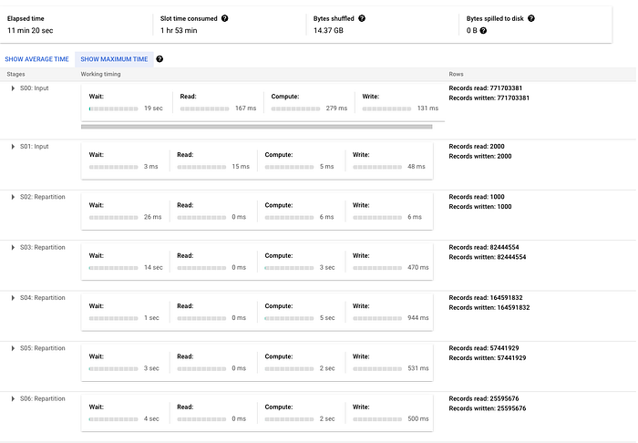
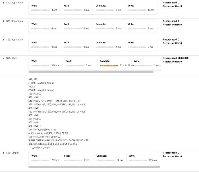
To illustrate this I am running a very simple merge statement to insert when no match is made on the transactions table in the crypto_bitcoin public dataset. I am merging a subset of the table consisting of one year of transactions with the full set of transactions (about 400GB and 1.54TB respectively). In this example, shown below, you will notice it has to do a lot of repartitioning of data between phases and then the bulk of the time is in a JOIN operation. Note that if this was a more complicated merge these phases would definitely grow more expansive as well and have more repartition phases as well.

Here is the outputted execution plan doing this (broken into two screenshots as it is quite large to prove the point):

Up Next
This concludes the second part of this series and is the last section of doing some mostly theoretical work. The next section will be actually looking at your BigQuery metadata and analyzing it.

Other parts in this series:
Part 1
Part 3