TL;DR: Amazon SageMaker offers an unprecedented easy way of implementing machine learning pipelines, significantly shortening the time to market for data scientists and engineers.

The NYC Taxi and Limousine Commission publishes detailed information regarding taxi rides in the metropolitan area. These data have been the subject of many data-science projects and several Kaggle competitions. In this tutorial, I am going to build a service that predicts future ride fare based on the origin, destination, and time of pickup. A service with similar functionality is probably implemented in most ride-hailing companies and the general idea can apply to additional geospatial prediction problems.

Imagine this, you work for one of the major ride-hailing companies, such as Uber or Lyft, as a data scientist. You are required to develop a prediction service that estimates the expected ride price (set by a meter) when given the following raw features: pickup and drop-off coordinates, pickup date-time, and number of passengers expected to go onboard.

Using machine learning, you will be able to build an accurate prediction model. This will, however, require massive amounts of data for training.

The strategy for solving the described problem includes the following 5 steps:

1. Explore the data
2. Build a dataset
3. Train a model
4. Evaluate the model
5. Deploy to production (monitor and refine)

The described strategy can be used by many software companies when encountering similar Kaggle-like problems. However, while these problems can be solved using a standard out-of-the-box machine learning pipeline, the majority of companies that I talk to spend a considerable amount of time implementing their own version of this very standard pipeline, thus wasting many developers’ hours.

If, for some reason, your team is developing this kind of service on AWS, you should really stop and read this article because it will save you weeks of coding and devising multiple iterations. Believe me, I’ve been there!

With Amazon SageMaker, it is relatively simple and fast to develop a full ML pipeline, including training, deployment, and prediction making. Announced in November 2017, Amazon SageMaker is a fully managed end-to-end machine learning service that enables data scientists, developers, and machine learning experts to quickly build, train, and host machine learning models at scale[1].

Full code following this tutorial can be found here:

https://github.com/doitintl/ML-on-Cloud-Examples/blob/master/SageMaker/taxi_fare_prediction.ipynb

For this exercise, I have used a dataset that was published here by Google, from which I extracted approximately 50M records (rides) between 2011 and 2015.

Step 1: Explore The Data

As always, the first step in building a machine learning pipeline is exploring the dataset. To do this AWS offers SageMaker’s notebook tool, which is a standard Jupyter Notebook server, preinstalled with all the swiss-knife python packages for data scientists.

After uploading the dataset (zipped csv file) to the S3 storage bucket, let’s read it using pandas. As mentioned above, the file contains over 50 million records, making it a complicated task for a single machine to process. Also, loading all the data to the machine’s memory requires an expensive instance with large disk and memory capacities. In my opinion, for the purpose of data exploration, using ~100K records is enough in this case. Working with such an amount of data generates valid statistics on the one hand, but also enables to query the data rapidly on a relatively low-cost machine.

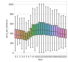
A few important insights I got from the quick EDA I performed, is the importance of time features. As you can see, the price per distance varies dramatically by the hour of day.

Another insight was related to the contribution of airports to the NYC taxi business. When generating a scatter plot of the pickup and drop-off coordinates, LaGuardia and JFK show strong figures.

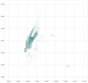
These insights are very frequently mentioned when analyzing the NYC taxi data. More on this topic with further insights can be found on Kaggle competition and in this blog post.

Step 2: Build A Dataset

Following the insights from the data exploration part, I’ve decided to extract the following features:

1. Sequential/categorical time: day, weekday, month, year, day-of-month, hour, minute
2. Cyclical time: sin/cos of day and week frequency
3. Distance: geometric distance
4. Airport distance: pickup and drop-off distance from JFK, LaGuardia, and Manhattan
5. Raw features — coordinates and passenger count

Calculating these features on the entire dataset requires the use of distributed computing and storage techniques.

Amazon AWS offers several tools to handle large csv datasets with which it is possible to process, inquire, and export datasets quite easily. I have used AWS S3 to store the raw CSV, AWS Glue to partition the file, and AWS Athena to execute SQL queries for feature extraction.

With regard to splitting the dataset to train and test, I considered two options:

1. Run two queries, using a WHERE clause to create different datasets over different periods; or,
2. Run one query to create a partitioned dataset and use the AWS-cli s3 command to move different partitions to new paths.

While in production systems, you would much rather use the first option, for the purpose of this exercise, the second option worked just fine.

Note: In the code that transforms partitioned csv to a libsvm, whoever implemented SageMaker forgot to use the partitions as features. So, when I partitioned by year and month — I actually lost information. To avoid this, you can work around it by adding the partition columns explicitly.

Step 3: Train A Model

Finally! Here is the best part of Amazon’s SageMaker.

After exploring the data and extracting features, I can start fitting a learning algorithm to the data. For this task Amazon had implemented its own version of ten common algorithms and libraries including Tensorflow, XGBoost, and PyTorch. AND, if that’s not enough, one can always implement their own algorithm to run with SageMaker by containing it.

For this kind of structured data, with millions of records, my natural preference is to start modeling with XGBoost. Because of its optimization algorithm and underlying data structure, XGBoost can converge fast on CPUs, while processing several GB’s of data in RAM. However, XGBoost’s parameter tuning can be a little tricky, but with good experience you can hit a good start, minimizing the training time and avoiding overfitting. For the most accurate results, it is recommended to perform some kind of hyper-parameter optimization, which is also covered by SageMaker, but not by this post. :)

To finalize the argument as to why XGBoost was the library I picked, I’d mention that experiments on multiple datasets show very good results using XGBoost, close to neutral networks. Thus, when presented this type of data, you will always find some implementation of Gradient Boosting Machines in every winning Kaggle solution throughout the past few years.

Nevertheless, in data science, there is no other truth but numbers. So feel free to experiment with whatever library you wish and please let us know how it worked for you in the comments below.

To perform the training you will need 2 main objects:

1. SageMakers S3 input object — pointing at the partitioned csv train/val that we created in step 3. Notice that using distribution=’ShardedByS3Key’ enables us to shard the datasets across several machines, making training much faster, but also reducing the number of samples used for fitting the model.

s3_input_trains3_inpu  = sagemaker.s3_input(s3_data='s3://{}/{}'.format(bucket, path_train), content_type='csv',distribution='ShardedByS3Key')

1. A SageMaker’s estimator, built with an XGBoost container, SageMaker session, and IAM role. By using parameters, you set the number of training instances and instance type for the training and when you submit the job, SageMaker will allocate resources according to the request you make.

container = get_image_uri(boto3.Session().region_name, 'xgboost')
                          sess = sagemaker.Session()
                          role = get_execution_role()
xgb = sagemaker.estimator.Estimator(container,
                                    role,
                                    train_instance_count=4,
                                    train_instance_type=
                                    'ml.m4.xlarge',
                                    output_path=output_path,
                                    sagemaker_session=sess)

Once the model instance is created, configure it using a preset of hyper-parameters and submit a training job.

xgb.set_hyperparameters(max_depth=9,
                        eta=0.2, gamma=4,
                        min_child_weight=300,
                        subsample=0.8,
                        silent=0,
                        objective='reg:linear',
                        early_stopping_rounds=10,
                        num_round=10000)

xgb.fit({'train': s3_input_trains3_inpu, 
         'validation': s3_input_validation})

Now, believe it or not, we are (almost) done coding for today. Go to the SageMaker console to track the training process. You can enjoy watching the CPU load on your allocated instances as XGBoost spins your CPU at close to 100% of its capacity during the training period.

For the rest of this post, we will use SageMaker’s console to deploy the model and make it available for predictions.

Step 4: Evaluate The Model

The training outputs the model to an S3 bucket that we’ve defined. To generate prediction on new data including our validation set we need to “create” it by selecting the training job and clicking the “Create model” button on the dashboard. By following the instructions on the screen, it should be easy to complete the task.

Next, create a batch transform job, and use it to evaluate your cross-validation data. This data should not contain the target field (really AWS…?) so you will probably need to transform your data AGAIN to remove it.

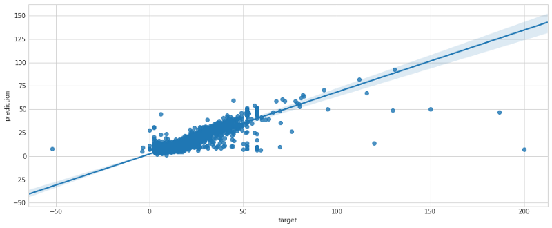
The results of the batch transformation showed low error, which after extended discussions with the management (remember you work for Uber/Lyft) was estimated to be low enough to go into production. Using seaborn’s regplot we show the error distribution on the cross-validation set.

Step 5: Deploy To Production

After evaluating the model and deciding that we’d like to expose it to our system, we need a way to generate online predictions. With the model stored in SageMaker, building a prediction service is as simple as it gets.

I will hereby show two possible ways of invoking the model:

1. Using a python boto3 client on an EC2
2. Making POST requests to an API

Both way require creating an endpoint configuration and an endpoint. Doing it is very simple, and once its done we can continue to make predictions using boto3 python client as such:

endpoint_name = 'taxi-fare-prediction'
content_type = 'text/csv'

runtime = boto3.Session().client('sagemaker-runtime')
response = runtime.invoke_endpoint(EndpointName=endpoint_name,\
                                    ContentType='text/csv',\
                                    Body=data)

results = list(ast.literal_eval(response['Body'].read().decode()))
print(results)

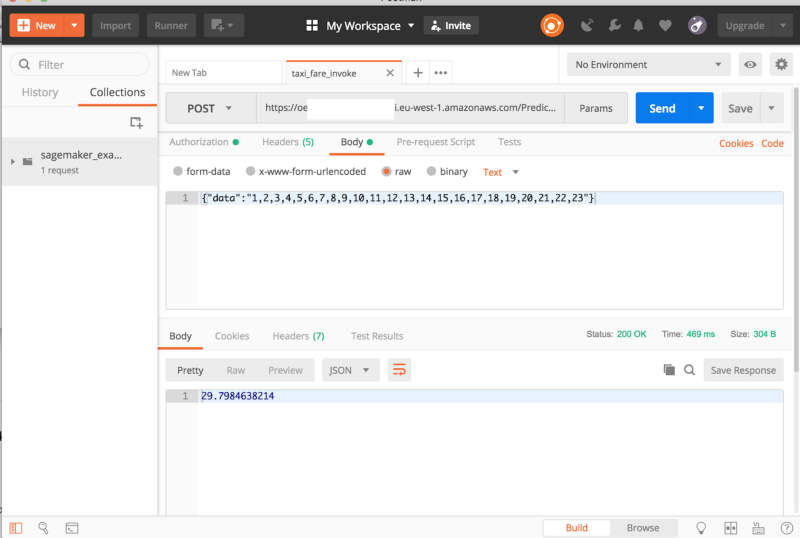
The second mentioned option, would be using a POST request. To expose it to external services, you can create an API Gateway, which invokes a Lambda function. Read more about it here.

In conclusion, AWS group has developed an amazing tool for building machine learning pipelines. Using SageMaker will shorten your time-to-market. However, it would be great if AWS could improve on data manipulation solutions and solve the minor issue with partitions.

[1] https://aws.amazon.com/blogs/aws/sagemaker/

Want more stories? Check our blog, or follow Gad on Twitter.